Introduction
This notebook does not produce a module to add to the library, it a place to run, and report on analyses using the library. It uses local code, shown below.
This is also an exploration of this style of presenting code, and data analysis based on it.
Geminga analyses
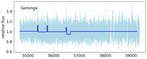
Following Kerr's example, we use the source Geminga to verify that this analysis of data gives results consistent with its being constant. As you can see below, the BB analysis finds several breaks, which merit further checks. That is followed by a simulation using Geminga's weight distribution and exposure. The run shown here finds one minor break, a change of 0.08%.
#from light_curves.tools import *
from wtlike.config import *
from wtlike.bayesian import *
from wtlike.lightcurve import *
from utilities.ipynb_docgen import *
config = Config(data_folder='/home/burnett/weekly')
source = PointSource('Geminga')
bba = None
plt.rcParams['savefig.pad_inches']= 0.1

def geminga_combined():
    """
    ### Cache contents for this source

    {geminga_cache}

    ## Fit to all data
    {outp}
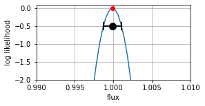
    This is the likelihood, for the combined dataset, a consistency check of the weight calculation.
    {fig1}
    """
    global bba
    with capture_print() as geminga_cache:
        print(config.cache.show( source.name))

    with capture_print('Analysis output') as outp:
        bba = BayesianBlockAnalysis(config, source)
        lla = bba.all_data_likelihood()

    #print(ll,'\nFit: ', ll.fit_info())
    fig1, ax1 = plt.subplots(num=1, figsize=(4,2))

    lla.plot(xlim =( 0.99, 1.01), ax=ax1)
    #fig1.savefig('test.png', bbox_inches='tight')

    return locals()
if config.valid:
    nbdoc(geminga_combined)
else:
    print('config not valid')
def analysis_plots(name, expect=0.9963, short=50, simname=''):
    """
    ### {sim} Geminga data

    {which_source} the daily binned data, or cells; then perform a Bayesian Blocks partition;
    finally make fits to the resulting blocks. <br>(Run at {date})

    {output}

    This shows the fits to all cells, with the BB fit overlays.
    {fig1}

    Since this is a constant source, there should be no breaks, that is, only one partition.
    Here is a table of the partition fits:

    {df_text}
    The last column represents the compatibility of the flux measurement for each partition
    with the expected value {expect} in equivalent sigma units.

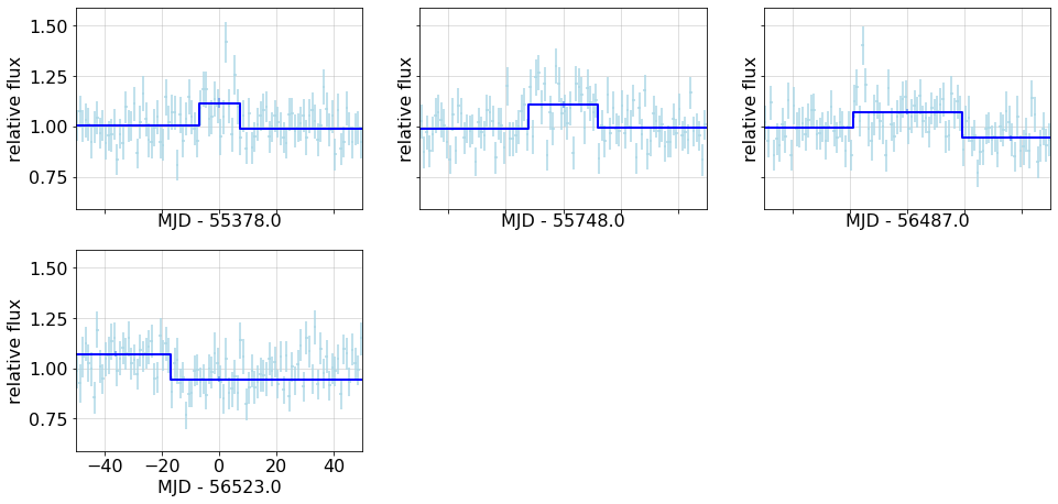
    Expand the plot around short, < {short} day partitions.
    {short_check}

    {fig2}
    """

    simulated = bool(simname)
    sim= 'Simulated' if simulated else ''
    which_source = 'Simulate a set of ' if simulated else 'Get'
    with capture_print('Analysis output' ) as output:
        if not simulated:
            lc = bba.lc_df
            bba.partition()
            bb_lc =  bba.bb_fit
        else:
            lc, bb_lc = simulation(config, source, bb_key=simname)

    pd.set_option('display.precision', 3)#, 'display.colheader_justify','left')

    df = fit_table(bb_lc, expect=expect)
    df_text = monospace(str(df), 'BB fit table', open=True)

    plt.rc('font', size=16)
    fig1, ax = plt.subplots(1,1, sharex=True, figsize=(10,4), num=1)
    bb_overplot(config, lc, bb_lc, ax = ax)
    ax.text(0.05, 0.85, name,  transform=ax.transAxes);
    fig1.width=600

    bb_short = bb_lc.query(f'tw<{short}'); ns =len(bb_short)
    if ns>0:
        short_check=f'There are {ns} such.'
        rows, cols = (ns+2)//3, 3
        fig2, axx = plt.subplots( rows,3,  figsize=(5*cols, 4*rows),
                                 sharey=True, sharex=True,
                     gridspec_kw=dict(top=0.85, left=0.08, bottom=0.15, hspace=0.2 ),num=2)
        if ns>1: fig2.width=600
        axf = axx.flatten()
        [ax.set_visible(False) for ax in axf[ns:]]
        for t, ax in zip(bb_short.t, axf):
            bb_overplot(config, lc, bb_lc, ax=ax, tzero=t, xlim=(-50, +50))
    else:
        fig2=''
        short_check = 'None found.'
    return locals()
if config.valid:
    nbdoc(analysis_plots, 'Geminga')
else:
    print('config invalid')
if config.valid:
    print('Simulation needs to be updated')
#     nbdoc(analysis_plots, 'Geminga', name='analysis_sim',  simname='analysis_plot_sim',
#          expect=0.9915)
else:
    print('config invalid')
TO DO
Fix a 0.4% bias from the cell fit when applied to high-statisics data.
Look at the intervals detected for the data, of which 5 have measured flux increases around 10%, more than 4$\sigma$. Possibilities are a problem with the exposure, and a change in the background. The latter can be examined by a 2-D fit with $\beta$ free. Another possibility, fixing $\alpha=0$ and fitting $\beta$ is not (yet) supported.


